A pre-amble:
MathML enables rendering of mathematical formulae directly in the browser without including external javascript libraries or inlined graphics. HTML5 contains the specification for MathML and thus ought to be supported by all browsers that have committed to HTML5. Unfortunately several browser developers seem to have decided that representation of mathematics on the web is not important enough to implement. As a work around I have also included MathJax versions of the equations. The following simple examples should make it clear whether your browser is rendering MathML correctly.
HTML5 native MathML:
MathJax javascript:
$$y={x+2 \over \sqrt{3} }$$
BMP085 Barometer at Low Pressure
Note that the BMP085 is now discontinued.
This experiment was initially intended to see how low a pressure I could achieve using a cheap, plastic, hand-operated vacuum pump. The answer turned out to be pretty low (of order 5% atmosphere, ∼50hPa) but the data sheet for my BMP085 barometer specified it operates 300 – 1100 hPa, so how realisitic are my measurements of 50 hPa?
The manufacturer's quoted absolute calibration errors, both worst case and typical, are given in the following table. There is no specification provided below 300hPa.
| 700–1100hPa 0 < T < 65°C |
±2.5hPa (typ. ±1hPa) |
| 300–1100hPa 0 < T < 65°C |
±3hPa (typ. ±1hPa) |
| 300–1100hPa -20 < T < 0°C |
±4hPa (typ. ±1.5hPa) |
Following the experiment described below, I believe the readings from this sensor are at least "ball park" accurate far below the specified 300hPa. A few points to remember though:
- I do not here present any absolute estimate of errors. I have not yet given any thought to how to achieve that. Suggestions are welcome.
- This sensor is designed as a pressure gauge, not a vacuum gauge. It is being used far outside its designed usage.
- It is possible that such low pressures could damage the sensor, though I have seen no ill effects after six months of operation.
- I have tested only a single device, and an obsolete design at that, though I suspect the newer devices perform similarly.
Theory
The ideal gas law describes the behaviour of an "ideal gas". At atmospheric pressure or below this is generally a very good approximation to the behaviour of most real gasses, including air.
where P is the gas pressure, V is the vessel volume, n is the quantity of gas, R is the universal gas contant (8.314 J K−1 mol−1) and T is temperature.
Part 1: Measure pressure as the temperature is varied
Here I will plot the measured pressure in a sealed, rigid, air-tight vessel as the temperature is changed. Rearranging the gas law equation gives P = (nR/V) T. Since the vessel is of fixed size and air-tight, both the volume (V) and quantity of gas (n) are constants, making (nR/V) a constant and
For a fixed quantity of gas in the jar, a plot of P vs. T is a straight line. Reduce or increase the temperature and the pressure must also reduce or increase in direct proportion. We do not care how much gas there is, just that it is constant throughout our experiment. This result is easy to verify empirically. Seal the barometer inside a jar with a thermometer and measure the pressure as the temperature changes. Plotting pressure vs. temperature should yield a straight line.
You can also imagine the opposite scenario. If you put a ballon in the freezer it will shrink because the balloon will try to keep the pressure inside it roughly constant and as the temperature falls, the volume will decrease. Warm it up and the gas expands again. The pressure inside the balloon would not be perfectly constant because of changes in the elasticity of the rubber, but it shows the point.
Part 2: Measure gradient of P/V relation as the quantity of gas is varied
Looking back at the ideal gas law and rearranging
That says the gradient of the P vs. T straight line is nR/V. We have fixed the volume V by always using the same jar and R is a constant anyway. That means the gradient is entirely defined by the absolute quantity of gas in the jar. The gradient is proportional to n. Double the amount of gas and the line will be twice as steep. We have no way of controlling the quantity of gas in absolute terms, but again rearranging the gas law we see
which tells us that if we hold V and T constant then n ∝ P. Therefore by running the experiment several times with differing amounts of gas, the slope of the P vs T plot in each data set is directly proportional to the pressure in that run at some fixed reference temperature. You can use any reference temperature you like so long as it is the same for each data set. All this works because the gas law is a simple straight line relationship that goes through the origin of the plot (P = T = V = 0).
The Experiment
Assuming the ideal gas law, we therefore have a way of testing if the sensor is still behaving linearly when we operate it far outside its specified range. The gas law predicts the form of the scaling laws as we vary either the temperature (keeping everything else constant) or vary the quantity of gas (keeping everything else constant). We plot these scaling relationships at pressures where the manufacturer specifies the sensor is accurate (>300hPa), pump out some of air and plot again. If the the sensor still follows the ideal gas law, we know it is still accurately reading the pressure. The lower the pressure, the more like an ideal gas air will behave so if at some point we see the gas appear to stop behaving like an ideal gas, we can deduce that it is in fact the sensor misbehaving.
The predictions to test are:
- With a fixed volume, plot of P vs. T always yields a straight line
- Extrapolating that straight line to temperature absolute zero would gives P=0. This is where the ideal gas law breaks down. At absolute zero temperature the gas would not disappear, but also it would likely not even be a gas anymore. Within the precision of this experiment we expect the line to go very close, but not quite through the plot origin at P = T = 0.
- A plot of the gradients in the above data samples against the pressure at a fixed temperature should also be a straight line. Any curvature in this plot would imply failure of the above samples to all converge to the same value at absolute zero.
Note that these are not independent tests. They are simply different ways of replotting and looking at the same data. If the first two are true (P vs T plot is a straight line that goes through the P = V = T = 0 origin) then the third has to also be true. On the other hand, if the straight lines do not all extrapolate perfectly to the origin, this last plot might make it easier to see if there are any systematic trends between the data sets.
Equipment and Procedure
A single BMP085. Obsolete. Ultimately I hope to repeat this experiment with the updated model.
I will not give much detail of the electronic setup. I read the devices using a JeeNode SMD, a small, low power, Arduino-like, ATMega328P board with an integrated RFM12B radio module, making it very easy to send measurements out to an external data logger. Measurements were logged into a MySQL database via the EmonCMS data logging system developed by the Open Energy Monitor project. The test vessel was a two US quart widemouth Ball jar with a ThiftyVac valve installed in the two-piece lid. All seals were smeared with a silicone grease before assembly. Everything was powered from four AA NiMH cells.
Procedure was to use the ThriftVac hand pump to evacuate the jar down to roughly the minimum operating pressure of the BMP085 (300hPa) and then record temperature and pressure as the jar was placed in the fridge, freezer and room temperature. Data points were logged only when the thermometer reading was stable, not while the system was equilibrating. A small amount of air was then pumped out and the thermal cycle repeated. This was repeated until the hand pump was no longer able to evacuate more air.
Results
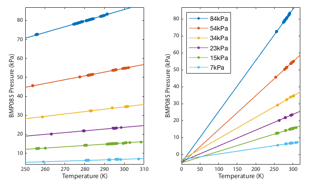
As shown in figure 1, the relationship between pressure and temperature during each thermal cycle was consistently linear for all data runs. The extrapolation to absolute zero temperature does indeed pass close to zero pressure. The deviation from perfect zero could be either a detection of the fact that air is not in fact a perfect ideal gas or a calibration offset in the sensor. All the line fits converge at a single point and there is no tendency for out-of-spec data (<300hPa) to diverge away from the in-spec data.
If the sensor were failing we might expect to see non-linear correlations or systematic relation between pressure and the extrapolated zero point intercept. We do not. The zero point intercept remains consistent.
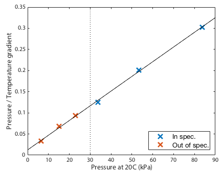
The final prediction was that the gradients should be directly proportional to the the quantity of gas, or since the volume is fixed, the gradients should be directly proportional to the pressure at some standarised temperature. This is clearly demonstrated in Figure 2. Since the fits in figure 1 converge near zero, this plot must be close to a straight line. Any curvature in this line would suggest that the failure of the fits to converge perfectly on a single spot was a systematic effect not just experimental noise. Given that the data points scatter randomly around a perfectly straight line, we see no evidence for systematic drift in the barometer calibration down to the limit tested.
Conclusions
In conclusion then, the gas still appears to be behaving to good approximation as an ideal gas even at 55hPa, -12°C. That is only possible if the baromter is still delivering reasonably accurate output, close to an order of magnitude outside the device's specified operating range.
Acknowledgments
Though I designed and integrated the entire experiment, I must acknowledge the many open source projects, both software and hardware, that I used.
- Jeelabs produce the JeeNode micro-controller board
- I developed my software using the Arduino tools and environment.
- My data logger is EmonCMS from the Open Energy Monitor project running on an Apple Mac.
- The plots and numerical analysis were generated in Octave.
- MySQL database.
- Apache web-server.
If you have comments or suggestions feel free to contact me:
2022-04-24 8:42 AM